
This is the first chapter of physics from the new NCERT textbook “Exploration” for grade 9. This is the most basic chapter of physics, the concepts of which you will apply in the subsequent chapters.
Therefore, you will need a to-the-point, clear, and condensed form of the concepts to master Describing Motion Around Us, Ch 4 Class 9.
And we have created “Describing Motion Around Us Notes Ch 4 Class 9”, keeping that in mind.
But to get the most out of these notes, you first should read the chapter thoroughly from the Class 9 Science textbook.
Then revise describing motion around notes, Chapter 4, Class 9, again and again.
Happy Learning!
Motion in a Straight Line
What is linear motion?
● Motion along a straight line
● Simplest kind of motion.
Examples:
- Swimming race
- A vertically falling ball
- A car moving along a straight highway
Describing position
● To describe a position, first fix a reference point
● Position = distance + direction from the reference point at a given instant.
Motion vs Rest:
Motion
position changes with time relative to the reference point.
Rest
position does not change with time relative to the reference point
Origin and sign convention
● The reference point is marked as origin O on a straight line.
● Only two directions in straight-line motion — forward and backward.
● Direction is shown using + and − signs.
Sign convention
Positive (+)
positions to the right of Origin(O).
Negative (−)
positions to the left of Origin(O)
Instant of time vs Time interval
Instant of time
A single clock reading at one specific point in time.
Time interval
The duration between two instants; the gap between two clock readings.
Distance travelled and displacement
Distance travelled
The total path length covered by an object.
Only the numerical value, no direction
SI unit: metre (m)
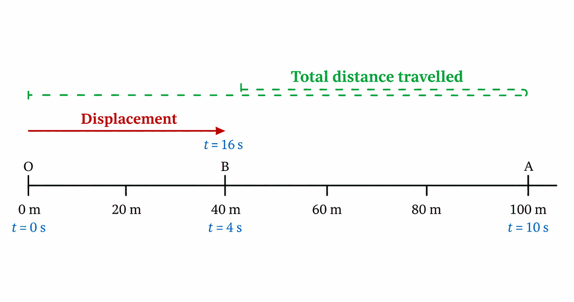
Example:
- Athlete runs from O → A → B (back)
- OA = 100 m, AB = 60 m
- Total distance = 100 + 60 = 160 m
Displacement
Net change in position
Both direction + magnitude
Magnitude
Distance between the object’s positions at the two instants.
Direction
From the position at the first instant to the position at the second instant.
SI unit: metre (m)
Example: Displacement = Final position – Initial position
From the diagram above:
Initial position = 0 m
Final position = 40 m
So,
👉 Displacement is 40 m in the positive direction.
Distance vs Displacement
| Basis | Distance | Displacement |
|---|---|---|
| Definition | Total path length covered | Net change in position between two instants |
| Direction required | No | Yes |
| Type of quantity | Scalar | Vector |
| Value | Always positive | Can be positive, negative, or zero |
| Depends on | Actual path taken | Only start and end positions |
| SI Unit | Metre (m) | Metre (m) |
| Can they be equal? | Yes, when motion is in a straight line without turning back | Yes, same condition |
Average speed and average velocity
To describe how fast or slow the object is moving
Average speed
Tells us how fast or slow an object moves.
Average speed =
Total distance travelled
÷
Time interval
● No direction
● SI unit: metre per second (m/s or m s⁻¹)
● Also measured in km/h (km h⁻¹)
Uniform vs Non-uniform motion
Uniform motion
● Equal distances in Equal intervals of time.
● Constant speed.
Non-uniform motion
● Unequal distances in Unequal intervals of time.
● Speed is increasing, decreasing, or a combination of both.
● If distances in successive intervals are increasing → speed is increasing
Limitation of speed
1. No information about direction.
2. Direction is also needed for a complete picture in many cases.
Average velocity
Describes how fast the position is changing and in which direction.
Requires both magnitude and direction
Direction of velocity
=
direction of displacement, shown by + or − sign.
Average velocity = Displacement ÷ Time interval
Rate of change
- Rate of change = change in a quantity ÷ corresponding change in time.
- Average velocity = average rate of change of position with respect to time.
Average acceleration
What is the average acceleration?
When velocity changes, the object is said to accelerate.
Average acceleration = Change in velocity ÷ Time interval
u = initial velocity at time t₁
v = final velocity at time t₂
a = average acceleration.
Requires both magnitude and direction
SI unit: m/s² or m s⁻²
Direction of acceleration
● If the magnitude of velocity is increasing → acceleration is in the same direction as velocity.
● If the magnitude of velocity is decreasing → acceleration is in the opposite direction to velocity.
What causes acceleration?
- Change in the magnitude of velocity, or
- Change in the direction of velocity, or
- Both together.
Constant acceleration
If the magnitude of velocity increases or decreases by equal amounts in equal intervals of time, acceleration is constant.
Acceleration due to gravity
- A special constant acceleration caused by the gravitational force of the Earth.
- Denoted by g.
- g = 9.8 m s-2
Graphical Representation of Motion
Plotting graph
Why use graphs?
Graphs give a visual representation of how position, velocity, and acceleration change with time.
Useful for:
- Comparing the motion of two objects.
- Calculating physical quantities.
- Identifying uniform or non-uniform motion.
Plotting a Position-Time Graph
Setting up the graph
- Draw two perpendicular lines — their intersection is the origin O.
- x-axis (OX) — horizontal line → plot time along this.
- y-axis (OY) — vertical line → plot position along this.
Choosing a scale
- Choose a scale that fits all data conveniently within the graph paper.
- Example scale:
- x-axis: 5 divisions = 1 s
- y-axis: 5 divisions = 20 m
Plotting points
- Mark time values (1s, 2 s, …) along the x-axis.
- Mark position values (20 m, 40 m, …) along the y-axis.
- For each data point:
- Draw a line parallel to the y-axis from the time value on the x-axis.
- Draw a line parallel to the x-axis from the position value on the y-axis.
- Mark the intersection — that is your plotted point.
- Repeat for all data points from the table.
Example data (Table 4.3 NCERT)
| Time (s) | 0 | 1 | 2 | 3 | 4 | 5 | 6 |
|---|---|---|---|---|---|---|---|
| Position (m) | 0 | 20 | 40 | 60 | 80 | 100 | 120 |
Result
- Connect all plotted points.
- For the data above, the result is a straight line — this is the position-time graph.
Position-time graphs
What does a position-time graph show?
● Shows how the position of an object changes with time.
● The shape of the graph tells us the nature of the motion.
Shape of the graph
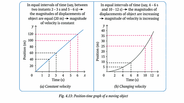
Straight line
● Object moves with constant velocity.
● Motion is uniform.
Curved line
● Velocity is not constant.
● Object is in accelerated (non-uniform) motion.
What can you find from a position-time graph?
- Position of the object at any instant of time.
- Average velocity — by reading positions at two instants and applying:
Slope of the position-time graph
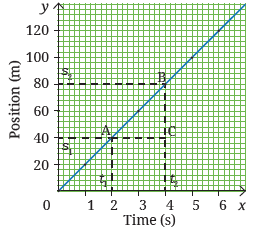
- Slope = steepness of the line on the graph.
- Geometrically, the slope of line AB:
- The slope gives the rate of change of position with respect to time.
- Therefore, the slope of a position-time graph = the magnitude of velocity.
Key points about slope
Steeper slope
→ higher velocity.
Gentle slope
→ lower velocity.
Straight line
→ constant slope → constant velocity.
Changing slope (curved)
→ changing velocity → acceleration.
Velocity-time graphs
What does a velocity-time graph show?
Shows how the velocity of an object changes with time.
Shapes of the velocity-time graph
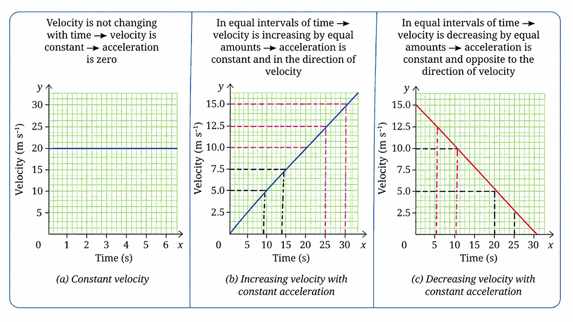
Straight line parallel to the x-axis
● Velocity is constant.
● Acceleration = zero.
Straight line going upward
● Velocity is increasing at a constant rate.
● Constant acceleration in the same direction as velocity.
A straight line going downward
● Velocity is decreasing at a constant rate.
● Constant acceleration in the opposite direction to velocity.
What can you find from a velocity-time graph?
- Velocity of the object at any instant.
- Acceleration — from the slope of the line.
- Displacement — from the area under the line.
Slope of the velocity-time graph
- Slope = rate of change of velocity with respect to time = acceleration.
Where u = velocity at time t₁, v = velocity at time t₂.
Key points: velocity-time graph
- Slope = 0 (horizontal line)
- → velocity is constant → acceleration = zero.
- Positive slope
- → velocity is increasing → positive acceleration.
- Negative slope
- → velocity is decreasing → negative acceleration.
Area under the velocity-time graph
The area enclosed between the graph line and the time axis = displacement in that time interval.
For constant velocity (rectangle):
Kinematic Equations for Motion in a Straight Line with Constant Acceleration
Conditions
- These equations apply only when acceleration is constant.
- Since acceleration is constant, acceleration at each instant = average acceleration.
Variables used
- u = initial velocity (at t = 0)
- v = final velocity (at time t)
- a = acceleration (constant)
- s = displacement
- t = time interval
1. First equation of motion
Starting from the definition of acceleration:
Starting from the definition of acceleration:
Gives the final velocity at any time t.
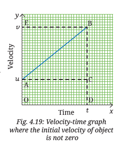
2. Second equation of motion
Using the area under the velocity-time graph:
Displacement = area of rectangle OACD + area of triangle ABC
Substituting (v − u) = at :
Gives displacement when time is known.
3. Third equation of motion
Eliminating t by substituting
Gives the final velocity when time is not known.
Motion in a Plane
What is motion in a plane?
Motion in a plane = motion in two dimensions.
Examples:
- A vehicle overtaking another
- Path of a kicked ball
- Satellite moving in a circular path
Uniform circular motion
What is circular motion?
When an object moves along a circular path, it is called circular motion.
Distance vs displacement in circular motion
● Distance travelled = length of the curved path (arc).
● Displacement = straight line between start and end points.
● These are not equal in circular motion.
For one complete revolution:
- Distance = circumference = 2πR (where R = radius)
- Displacement = zero (object returns to starting point)
Average speed in circular motion
- Where T = time taken for one revolution.
- Average velocity over one full revolution = zero (since displacement = 0).
Uniform circular motion
When an object moves in a circular path with constant speed, it is called uniform circular motion.
- Speed is constant, but the direction of velocity changes continuously.
- Therefore, velocity is not constant.
Why is uniform circular motion accelerated?
● Acceleration = change in velocity
● Velocity changes if direction changes.
● In uniform circular motion, direction constantly changes.
So, it’s always accelerating.
Understanding the continuous change of direction
- Rectangular track → direction changes 4 times per round.
- Hexagonal track → direction changes 6 times per round.
- As the number of sides increases → direction changes more frequently.
- At infinite sides → path becomes a circle → direction changes continuously